Proxima Centauri: The Star-Next-Door with Flair

Title: Most Observations Of Our Nearest Neighbor: Flares On Proxima Centauri
Authors: James R. A. Davenport, David M. Kipping, Dimitar Sasselov, Jaymie M. Matthews, and Chris Cameron
First Author’s Institution: Department of Physics & Astronomy, Western Washington University, Bellingham, WA, USA.
Status: Published 2016 September 29 by The Astrophysical Journal Letters;
Available at: https://arxiv.org/pdf/1608.06672.pdf

In August 2016, Astronomers made the ground-breaking discovery of Proxima Centauri b, an Earth-mass planet in the temperate zone of Proxima Centauri, the closest star to our Sun. The discovery has been effective in fueling the hope that the long-sought “Another Earth” might exist around the Sun’s nearest neighbor.

One problem, though. Our nearest stellar neighbor seem to have a flair for the dramatic.

Seasoned in the Flare Scene

In today’s paper, Davenport et al. utilized the Canadian micro-satellite Microvariability and Oscillations of STars (re: MOST) to study white-light flares emitting from the active M5.5 dwarf, Proxima Centauri over the course of 37.6 days.

The paper first emphasized the challenges Stellar magnetic activity posed to the questions of habitability and detectability in M Dwarfs like Proxima Centauri. Stellar magnetic activity is present in surface activity such as flares, and their role has been a topic of growing interest in assessing planetary habitability.

They then noted that, in spite of these challenges however, our nearest neighbor Proxima Centauri has long been an active flare star, and that’s important because of the great potential in using her as a model in better understanding flares.

Furthermore, given astronomers’ recent discovery of Proxima Centauri b, its host star has become integral in understanding planet formation around low-mass stars, the evolution of the magnetic dynamo, and the impact of stellar activity on planetary atmospheres.

Following the (White) Light

Flares have been previously studied with MOST before; however, very few other mid-to-late M dwarfs are bright enough or located within acceptable viewing zones to be studied as Proxima Centauri is.

Indeed, she’s special, and with the aid of MOST, researchers now had an unparalleled ability to statistically characterize rates and energy distributions for stellar flares.

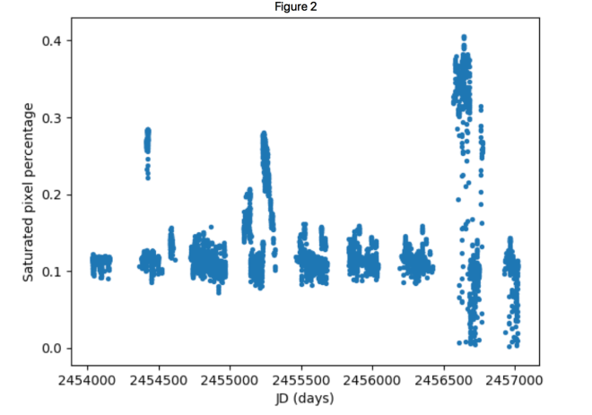
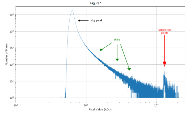
The data Davenport et al. presented on Proxima Centauri came in the form of light curves from two observing seasons with MOST, shown in Figure 1 below.

But what about all of these squiggly lines? Well, it shows us how these researchers identified white-light flares— in the form of data points above a smooth light curve showing us the duration of these flares, and analyzing them in fractional flux units showing us decays in brightness.

In their study, Davenport et al. identified a total of 66 flare events between the two— the largest number of white light flares observed to date on the star— finding  constant flare rate between both seasons, as well as the average amount of flares per day. The figure below shows the cumulative flare frequency distribution (FFD) versus event energy, which is the typical parameter space used to characterize stellar flare rates.

Ultimately, Davenport et al. concluded that the flares in their sample spanned more than 2 orders of magnitude in energy, and that Proxima Centauri showed an unusually high flare activity given its slow rotation period.

Fitting the Flair for Proxima b.

So where does all this flare-talk fit in the context of the new exoplanet next door?

Well, if you’re on the hunt for any sign of extraterrestrial life, you should totally care about Proxima Centauri’s flares, since they can reveals to us whether dwarf flares pose a risk to general planetary habitability.

And you know those 2 orders of magnitude? Well, they’re pretty significant too, and they have posed a great dilemma for researchers. These orders encompass the nature of two varying kinds of flares observed on the star.

“Our flare rate indicates Proxima Cen could produce ∼8 superflares per year at its present age, and 63 flares per day with amplitudes comparable to the transit depth expected for Proxima b. Comparing our flare rate to other M5–M6 stars suggests Proxima was more active in its youth.” (Davenport et al.)

The “small” flares which occur on the daily have energies on the lower magnitude while minority (but by no means minor) “superflares” occur on the upper magnitude, with energies approximately at 10^33 ergs.

Now, is one more favorable than the other? And how do these relate to habitability?” you may ask.

Both questions pose quite the dilemma for researchers and astro-enthusiasts alike, as either flares presents some sort of challenge. Small flares, for instance, are pretty hard to work with if one  wishes to rely on them to find transits like moons around Proxima Centauri b. Superflares, on the other hand, may be especially difficult for alien hunters to grapple with, as they could have a significant impact on the planetary atmosphere, thus literally zapping all hopes of finding Another Earth.

A flair for the dramatic indeed, huh, Proxima…

The researchers concluded their paper by stating the role Coronal Mass Ejections associated with flares may play in impacting Proxima b’s habitability, underscoring that any planet that were being frequently bombarded with such CMEs would see a significant compromise in the survival of its atmosphere.

Whether you appreciate our stellar neighbors’ flair of flaring is up to you, and whether its newly discovered tenant, Proxima b, appreciates her outbursts will, hopefully, be the topic of a future studies and (perhaps even) future Planetbites article!

Sources:

https://arxiv.org/pdf/1608.06672.pdf

Breaking Down the Accuracy of Kepler’s Exoplanet Detection- The Legitimacy of Kepler-452b

Title: KEPLER’S EARTH-LIKE PLANETS SHOULD NOT BE CONFIRMED WITHOUT INDEPENDENT DETECTION: THE CASE OF KEPLER-452b

Authors: Fergal Mullally, Susan E. Thompson, Jeffrey L. Coughlin, Christopher J. Burke, and Jason F. Rowe

Link: https://arxiv.org/pdf/1803.11307.pdf

Kepler Telescope

The Kepler astronomical observatory has been discovering exoplanets in distant galaxies since, but not every discovered planet can be confirmed based on Kepler data.  For Kepler, the accuracy of its discoveries depends on the detected planets’ periods.  Using data from measured periodic signals, Kepler is responsible for the confirmed discoveries of many small, short-period exoplanets using radial velocity detection.

However, Kepler is limited in its ability to confirm planets with longer periods of over 200 days.  Confirmation of these small planets cannot happen only using data from the Kepler telescope.  Kepler-452b is a prime example of a “discovery” of Kepler that was disputable by researchers because of its longer period.

What is Kepler-452b?

Kepler-452b was identified in 2015 by the Kepler telescope, and it is 1400 light years away from our solar system.  It is believed to be habitable, with rocky features and similar temperatures to earth.

To try to confirm the planet-hood of Kepler-452b, along with other small, long-period exoplanets alike, researchers use the technique of statistical confirmation.  Authors Mullally, Thompson, Coughlin, Burke, and Rowe argue that even this technique has its limits.  With both data from Kepler and from statistical confirmation, it is argued that Kepler-452b and other similar planets cannot be confirmed using this technique that was thought to be accurate.

To give a background of the method of statistical confirmation, the calculation is below.  Using planet period and the probability that the received signal is from an eclipsing binary, statistical confirmation is usually accurate.  However, complications occur when planets’ periods are over 300 days.  The second equation shows a factor that must be included when considering these long-period planets- the probability that signals detected a non-astrophysical signal.

 

These “false alarms” are very common among discoveries of small planets with long periods, and are often indistinguishable from planets to the eye.  Kepler-452b is viewed as the best specimen for the inaccuracy of statistical confirmation because out of the many long-period planets with confirmed confirmation, Kepler-452b has the lowest signal-to-noise ratio, or SNR.  The criticism of statistical confirmation has caused Kepler-452b, a planet that has been deemed habitable, to be questioned about its identity as a planet.

To be confirmed, a planet must have observed signals (TCEs) that signify a planet with 99% confidence.  A Threshold-Crossing Event (TCE), by definition, is a “sequence of transit-like features in the flux time series of a given target that resembles the signature of a transiting planet to a sufficient degree that the target is passed on for further analysis” (NASA Exoplanet Archive).  So when Kepler detects a TCE, the chances are that the signal did not come from a planet.  An overview of TCEs, planetary candidates, and specifically Kepler-452b, detected by Kepler is seen below.

As shown in the diagram, many discrepancies registered as TCEs are picked up by Kepler, and Kepler-452b sits among them with very similar orbital period and Multiple Event Statistic (MES).  In the case of all the planetary candidates shown in the distribution by blue circles, all of them have one thing in common- their probability that signals were picked up via an astrophysical event are too low to be considered confirmed.  That being said, without more evidence observed.  As stated by the authors, “We leave the analysis of these systems as future work” (Mullally et al.).

In conclusion, Kepler is apt in its purpose of detecting exoplanets, but has its limitations when trying to detect planets of small size, low SNR, and long period.  Kepler‘s discovery of Kepler-452b gave researchers the notion that there was a habitable planet in a distant galaxy, but further research questioned the planet-hood of Kepler-452b.  This shows the importance of research- discoveries in the universe are not always accurate, and there is always more information to be uncovered.

Additional Source: https://exoplanetarchive.ipac.caltech.edu/docs/Kepler_TCE_docs.html

Another Earth… Literally

Article: Life could Survive on Earth-sized moons of gas giant exoplanets

Author: Andrew Grant

http://www.jstor.org/stable/pdf/23598839.pdf?refreqid=excelsior%3A75da6b53a4ea4ddf8f96c6dcaea45572

 

Us Earthlings are always on the hunt for other habitable planets in some far away galaxy. We want to expand our world, or escape to a new one. But what if what we’ve been looking for all along was in our own galaxy? According to Astronomer reports in Astrobiology, Earth-sized moons in galaxies trillions of miles away could be the breeding grounds for alien life. So far, there have been thirty-six hundred confirmed planets that are orbiting other stars. While this seems like great news, as we may know, in order for a planet to be habitable, there are temperature and size conditions that need to be met, none of which have been by these planets. Of those planets, more than 150 are gas giants and could potentially have liquid water, which is a solid start, but still no ground to walk on, so we still have an issue. If we take a look within our own solar system, we can see that life could possibly survive on the rocky moons, similar to those of Neptune and Jupiter. In order to life to be sustained, there are many factors that contribute. The moon must orbit at the perfect distance from the planet but also from its star.  This is crucial because this planet will be hit with the radiation both from the star and from the planet through the reflection off of the clouds. This is also important because stars become more luminous as they age, and so this distance needs to be great enough that the planet can still maintain life over the course of many centuries. Let us not forget that moons undergo tidal heating, which causes them to become deformed through squeezing, causing them to warm up. While this could be a great source of heat, this also poses a threat to sustain life. If the moon is in constant squishing, is it really possible for humans to inhabit it?

We also would need to think about eclipses and how at any one point, only one side of the moon could have both the star and the planet in its view, eating up all of this energy, while on the other side (with the potential rest of population) was shrouded in darkness as explained in the image below. What would that mean for civilization? If only have of the moon will be receiving energy at any given time, will the moon itself absorb enough energy to sustain life? According to researchers, they do believe the moon would be able to sustain life in these harsh conditions. Astronomers Rene Heller of Germany’s Leibniz Institute for Astrophysics Potsdam and Rory Barnes of the University of Washington in Seattle have set out on their research to determine the habitability of exomoons.

.

Two major facts that we know are needed for habitation are an atmosphere to protect us from radiation and a magnetic field. In order for the moon to even be considered habitable, it needs to also have a certain mass, similar to Earths, in order to maintain the two key components. We tend to forget how large our planet is and so as a  comparison, one of Jupiter’s moons,Ganbymede, is only 2% as massive as earth so this requirement is not one easy to come by.

There are many ways for a planet to obtain a moon, as we have learned. One of which is through capture, using the planets gravitational pull as the moon is passing by its orbit. It is quite possible that planets, even if it is a gas giant with no solid surface, could have a great gravitational force and capture larger moons, in order to be considered habitable. Heller and Williams agree that of all the strange combinations of moons, stars, and planets, finding one with an appropriate mass that orbits a gas giant should be quite achievable. Barnes and Heller have both dedicated their time to combine all of these factors and create a measure called the Habitable edge, the minimum distance a moon needs to be from its planet to allow for life. This will ensure that the moon is not too close, causing it to be taken over by the forces acted upon it through tidal heating.  As we all should know, Professor Kipping has dedicated his life to the research of exomoons, and these new discoveries could definitely lead to an exciting future.

Discovering exomoons is no easy feat, and takes a vast amount of resources. Some of which that do not exist yet. Researchers need to take in many factors while considering a moon or planet, such as obtaining imaging of the body to begin with, which could prove to be a challenge. These moons are surrounded by the luminosity given off from nearby stars and this could interfere with the quality of data that is obtained. While this potentially won’t be an option in our lifetime, researchers are continuously creating new telescopes and are very confident that life as we know it does potentially exist somewhere else, and these discoveries are taking us one step closer to finding our “other” Earth.

Frosty the Snowball, Was a Very Habitable Planet!

Have you ever wanted to live on Antarctica? Me neither! So, what would make living on an ice-covered planet seem like such a good idea? Well, maybe not at the moment, but certainly in the future. There appears to be hope for ice-covered “snowball” planets after all.

It was previously believed that snowball planets were inhabitable because of their inability to nurture and maintain liquid water…and that pesky positive-feedback loop that keeps temperatures to extremely icy lows. However, there’s a catch! According to Earth’s history, it has been through two snowball periods. Earth is certainly habitable now, right? We are most certainly living it up on Earth’s crust, at least on the parts that aren’t the north or south poles (with the exception of Santa and his reindeer)!

The high albedo levels due to the sea ice can cause a snowball planet to maintain its icy cover even if it is hit with very high levels of greenhouse gases, or irregularly large amounts of sunlight. But there is hope! Earth seemed to return to temperate climates following its snowball periods. Additionally, there was no significant evidence of a loss of biodiversity. It would require lots of heating and melting–large increases in insolation and extreme levels of greenhouse gases might just do the trick. Maybe not enough to deglaciate an entire planet, but it is certainly possible for there to be habitable regions…which is still incredible, if you ask me!

The point that the authors are getting at is that it is not necessarily the case that low average global temperatures means a planet COMPLETELY covered in ice. The global averages don’t necessarily take into account some smaller regions that may contain warmer, habitable temperatures.

The Figure above displays an example of a hypothetical planet (centered on the equator) whose annual average surface temperature may signify a snowball planet, but which clearly shows a continent with a temperate, habitable climate. A planet such as this, with zero obliquity and a large amount of land on the equator may maintain a temperate climate, and therefore be habitable year-round.

The author claims that planets may be partially habitable or habitable at certain times of the year even when in a snowball period. He uses a General Circulation Model to show that this is possible for planets with high obliquity or high eccentricity. High obliquity would cause one part of the planet to have a lot more exposure to the sun than other regions. The same goes with high eccentricity– if a planet is very eccentric it means that at different times it will get more sun exposure than at others.

The discovery of possible habitability on snowball planets, even if not the entire planet, is a huge advance. As we continue our great quest for life on other planets, and for other habitable planets besides Earth, The infamous snowball planet is no longer a dud. It is rather, an opportunity for further exploration! This has expanded the original definition of what constitutes a “habitable’ planet.

Citation:

Click to access 1803.00511.pdf

Where do Phobos and Deimos come from?

Title: On the Impact Origin of Phobos and Deimos I: Thermodynamic and Physical Aspects

Authors: Ryuki Hyodo, Hidenori Genda, Sébastien Charnoz, and Pascal Rosenblatt

Status: Accepted to the Astrophysical Journal, open access

 

For many years astronomers debated just how Mars’s moons were formed. They originally believed they were the result of interplanetary kidnapping, but have recently decided that since they don’t have highly eccentric orbits that they could not have resulted from a kidnapping.

Many astronomers now believe that Mars’s two moons, Phobos and Deimos, are the result of a massive impact that occured 4.3 billion years ago. Unlike the original belief that they were a result of an interplanetary kidnapping, they could collect from the debris disk made by a possible impact, which is now a more believable theory.  

Figure 1. Topographical map of Mars. Borealis basin is the low-lying (blue) region in the northern hemisphere. It encompasses many officially-named regions, such as Vastitas Borealis and Utopia Planitia. Adapted from this image, which is made from data from the Mars Orbiter Laser Altimeter aboard Mars Global Surveyor.

 

In the paper, the authors talk about how they used SPH simulations (smoothed particle hydrodynamics) to learn more about the structural and thermodynamical properties generated in the speculated impact. SPH is a common method used when simulating astrophysical fluids, or systems with a large number of particles that can be treated as a fluid, like stars in colliding galaxies.

Figure 2. Snapshots from the first 20 hours after the simulated impact. Top row: Positions of particles over time. Red points are Mars particles, yellow are particles that fall on to Mars, white are disk particles, and cyan are particles that escape the system. Bottom row: Temperature of the particles. Shock heating in the moments after impact liquefies much of the material. Adapted from Figure 1 in this paper.

 

A key finding to this theory was that the disk contains material from a young Mars and the impactor. Regardless of the angle at which the two made contact, the disk contains approximately ~35% martian material by mass. As you go farther out in the disk, this number rises to about ~70%. And most of this material comes from the mantle of young Mars.

Figure 3. The cumulative fraction of Mars-originating disk particles as a function of the depth below Mars’ surface from which they originated. Beyond 4 Mars radii (solid line), there is a higher percentage of particles originating from > 50 km below the surface than in the disk as a whole (dashed line). Figure 4 in this paper.

 

Although the radial distance and angle of impact at which the moons form determine how much material from Mars they contain, all scenarios of formation lead to the moons being made of whatever the impactor was and martian mantle. This theory helps fill some of the gaps that were made with the original kidnapping theory, such as how did they get into orbit if most moons that resulted from kidnapping have an eccentric orbit.

 

Links:

What are Mars’ moons made of?

https://arxiv.org/abs/1707.06282

 

Measuring Atmospheric Mass Loss in the Exoplanet Age

Article: Atmospheric mass loss of extrasolar planets orbiting magnetically active host stars (https://arxiv.org/abs/1803.08684)

Authors: Lalitha Sairam¹, J. H. M. M. Schmitt², and Spandan Dash^3
1 Indian Institute of Astrophysics, II Block, Koramangala, Bangalore 560 034, India
² Hamburger Sternwarte, Gojenbergsweg 112, 21029 Hamburg
³ Indian Institute of Science, C.V Raman Avenue, Yeshwantpur, Bangalore 560 012, India

As the recent discovery of three Earth-like planets in the habitable zone of Trappist-1 attests, there exists an abundant supply of potentially habitable exoplanet candidates. Considering the importance of stable, non-volatile atmospheres for planetary habitability, exoplanetologists have dedicated considerable resources to tracking down and identifying the robustness of exoplanet atmospheres. Planets without sufficiently thick atmospheres provide little protection against high-frequency radiation and meteorite impact, as well as have poor heat transfer across their surfaces, making them unlikely to harbor the biochemical processes necessary for life.

That being said, the first extrasolar planet discovered to have an atmosphere, HD 209458 b, did not prove to be exactly what habitability-minded researchers had in mind. While the planet does have a rich atmosphere, that atmosphere is being constantly evaporated by its host star, leaving it with an incredible comet-like tail (see below). Though astronomers originally considered Jeans escape, whereby certain high-tail molecules acquire enough kinetic energy to reach the escape velocity necessary to leave a planet’s atmosphere, to be the predominant model of atmospheric loss, HD 209458 b, proved that there was another mechanism at work, namely hydrodynamic mass loss. This thermal escape system demonstrates that, given a large source of energy (think a nearby star!), planetary atmospheres can be essentially “blown off” as light atoms heat up, collide, and drag heavier atoms like oxygen and carbon into space.

Image 1. Artist’s rendering of HD 209458 b undergoing atmospheric loss. The escaping gas from the planet forms an envelop of carbon and oxygen that follows it like a tail.

Building off of these findings, Sairam et al. investigate the relationship between host stars and exoplanet atmospheres for five other well studied short-period hot Jupiters: Kepler-63 b, Kepler-210 b and c, WASP-19 b, and HAT-P-11 b. By estimating the coronal temperature and X-ray activity of these exoplanet’s respective host stars from new X-ray observations collected by the XMM-Newton satellite, they are able to calculate the individual rates of the planets’ hydrodynamic atmospheric mass loss and, subsequently, juxtapose these rates with those of hot Jupiters like HD 189733 b and of the planets of our solar system.

To understand the methodology of the authors, it is salient to first look at the XMM-Newton observations, which relate that the X-ray emissions emanating from the sample stars point to moderately active to active sites of stellar activity. Using extrapolated scaling relations for these stars, Sairam et al. are able to measure the stars’ X-ray luminosities and, from these calculations, derive their high-energy radiations. Subsequently, by making a series of assumptions about planetary heating efficiency and the radii of the planets, Sairam et al. obtain rough approximations about each planet’s individual upper-limit mass loss rates.

While the composition of the planets in study is not known (meaning that these density-based rates of mass loss might be proven inaccurate), Sairam et al. claim that changing extreme ultraviolet (XUV) flux is by far the most dominant component for accelerating atmospheric mass loss. Determining the age of the star is, thereby, critical because stellar activity is not constant over the lifetime of stars—for instance, large stellar rotation of the star following early solar contraction produces uncharacteristically high levels of activity. In Figure 1 below, we see a plot showcasing the potentially different mass losses that could arise at different ages of the WASP-19 system. If, for example, the star was 4  Gyr old, it would correspond to having caused approximately 2 M_J of total planetary mass loss. By comparing the X-ray luminosity of WASP-19, however, with the age-X-ray luminosity relations, Sairam et al. predict that the maximal mass lost by its planet is actually around 1 M_J , corresponding to a solar age of around 2.2 Gyr.

Figure 1. Progressive evolution of the total planetary mass loss of WASP-19 for the current X-ray luminosity. Notice that, regardless, of the sun’s potential age, most planetary atmospheric mass loss happens during its early stage of life, before plateauing off to a steady rate over time.

To better contextualize these findings, Sairam et al. go on to compare the five target extrasolar planets with the gas giants in our solar system, making the same series of assumptions as before. Figure 2 below indicates that the exoplanets have maximal mass-loss rates whole orders of magnitude higher than the gas giants, most likely because the latter orbit much further away from their star (our sun) and because the X-ray luminosity of our sun is much lower than that of the extrasolar planets’ respective host stars. Even when compared with the high mass loss rates of HD 209458 b and HD 189733 b, the five sample planets yield rates that vary from being on par to at least an order of magnitude higher.

Figure 2. On the x-axis: mass for solar system gas giants and sample exoplanets vs. on the y-axis: log M (upper-limit estimates of mass loss). Notice the drastic difference in mass loss between our solar system planets and those in the sample.

Needless to say, a more in-depth understanding of how these sample exoplanet atmospheres develop so close to their stars will depend on pinning down the XUV fluxes of their host stars and their compositions. Developing a better sense of how solar activity impacts atmospheric loss can, concurrently, offer more substantial insight into how to delineate the range of each star’s personal habitable zones. In order words, to not underestimate the actual atmospheric mass loss occurring, hydrodynamic mass loss must be taken into account as we continue our search for another earth.

Formation of Terrestrial Planets

Article: Formation of Terrestrial Planets

Authors: Andre Izidoro and Sean N Raymond

 

There is no doubt that human knowledge of the solar system has increased by leaps and bounds within recent history. However, many questions regarding the various complicated scenarios which determine the origin and coagulation of a planet remain completely unanswered. While the quest for life beyond earth proves to be one of the most significant driving factors keeping planetary study at the foreground of modern science, questions regarding what physically differentiates planets from one another and what conditions are driving this production is one of particular intrigue to scientists. Because of these very reasons, Andre Izidor and Sean Raymond were inspired to ask how we can understand our Solar System in a broader context in their study called “Formation of Terrestrial Planets.”

As of 2018, over 3,000 exoplanets have been confirmed in outer space, and that is only what we know of. A majority of these planets were discovered via observations of Doppler shifts in the realm of the planet – in – question’s parent star. This is also known as Doppler spectroscopy. However, much like animals, plants, and humans, no two planets are exactly alike. Within our solar system alone, we have a slew of names that signify one from another. There are terrestrial planets and protoplanets, ice planets and gas giants, and this is just the tip of the iceberg. Some planets, like Mars and Jupiter, we know a lot about. With others, we are only beginning to breach the surface of their wonder. In turn, Izidor and Raymond propose that getting to know our planets on an individual level might be the most effective way of coming to understand the solar system and even humanity at large.

This study particularly looks at the processes which take us from miniscule dust particles to the grand planetesimals which we know of today. In the earliest stages of development, a planet can consist of 99% gas and 1% dust, so what factors could possibly be occurring that can take a mere planetary embryo such as that to a gigantic planet? At this early stage, we know that gravity seems to play the biggest role in initiating planetary development. What starts as some sort of “accident” is then kick-started into gear by a combination of speed, motion, and friction. Once these tiny planetesimals are formed, one of two processes begin; accretion and/or collision. Next, velocity increases a planets collision probability which ultimately determines how big and fast they grow.

Our authors propose three scenarios which explain planetary growth and segment them into different growth regimes, runaway, orderly, and oligarchic. The following chart depicts planetesimal embryo growth during the “oligarchic” regime and shows how velocity affects the position and size of a planetary body.

While these three regimes could provide an explanation for what ultimately determines the mass, composition, and dispersion of a planet, what precisely differentiates these models remains debatable. Another question as to what makes the Solar System so unusual is the lack of super-Earths: a planet with a mass higher than our own. One explanation they suggest is that planetary involvement can prevent planets such as Uranus and Neptune from penetrating the inner solar system. A planet like Jupiter, they claim can be understood at the solar system’s “primary architect” and has affected the outcomes of many other planets. Here we being to see the relationship that planets have upon one another in terms of where they end up, their mass, and what kind of orbit they end up having.

This diagram offer a detailed depiction of the mass and orbital evolution of a group of 10 close-in super-Earth’s ending in a phase of collisions.

In the end, this study suggests that if we can begin to better understand planetary formation on a micro level, then we can ideally understand the formation of our solar system in a broader setting. The magnitude of discovered exoplanets provide an abundance of knowledge for us to study in order to make sense of these unbelievably complex systems of nature.

 

Planetseeds Reach for the Stars!

Title: The diverse lives of massive protoplanets in self-gravitating discs
Authors: Dimitris Stamatellos, Shu-ichiro Inutsuka
First Author’s Institution: Jeremiah Horrocks Institute for Mathematics, Physics & Astronomy, University of Central Lancashire
Status: MNRAS accepted, [open access] http://www.star.uclan.ac.uk/~dstamatellos/Publications_files/protoplanets.pdf

It is remarkable to think of the effects every detail of every cosmic event can have. Every celestial body we observe today, within our Solar System and beyond, was formed and shaped by the events that came before, out of the properties of the space it formed out of. Today’s paper uses a unique style of simulation to expound on the question, what made the exoplanets we detect today? What process did they come out of?  Specifically, the focus is placed on the case of the gas giant exoplanets more easily detected and commonly observed today.

Chronologically, Safronov, Goldreich & Ward, Mizuno, Bodenheimer & Pollack, and Pollack et al. have proposed a model of core accretion; they suggest a massive core, several times the size of the Earth’s, forms out of the coalescing of dust and space material over time. The resulting gravity of this core then draws in the envelope of gas. This model, however, is problematic in that the process it describes would take millions of years, outliving the circumstellar discs of most stars observed today, and failing to explain the peculiarly wides orbits of many of these planets.

Rather, this paper draws upon and gives support to a second theory, that these planets may also form out of the gravitational fragmentation of protostellar disks. This theory holds that, once a fragment forms inside of such a disk (assuming the disk is of a certain mass and gravity), it begins to move around, collecting gas, increasing in mass and causing a gap to open within the disk. It is hypothesized that if the resulting body is ejected near that point, it becomes a normal planet, of an accepted planetary size. If it continues within the disk, however, it may evolve into a gas giant, or continues to accrete at such a rate that it exceeds the mass-limit, or ignites deuterium, elevating its status to a brown dwarf. Such seeds are labeled ‘protoplanets’ in this paper’s study due to the mystery of their futures. Such a theory would be valuable because it would provide the basis for a more dynamic timescale for the planet’s formation (as short as 10,000 years), as well as explaining the formation of the wider-orbiting planets referenced earlier.

Whether or not such a process is possible, however, and whether or not the likelihood of a fragment surviving as a planet is convincing and robust enough to make this a reliable model, is explored in this paper’s computational simulations. The estimates used are conservative, at the lower bounds of what former papers deem necessary for disk fragmentation. The initial seed is estimated to be the size of Jupiter, and it is inserted into a stable, circular protostellar disk that has been at rest for ~3kyr.

The first simulation has five runs, wherein parameters are adjusted to account for variances in the protoplanet’s radiative feedback, the disk’s viscosity, inclinations in the protoplanet’s orbit around the central star, and factoring in “Seminov opacities”, or differences in the size and composition of particles within the disk.

Figure 3 (included below) demonstrates the changes in the protoplanet’s mass as the simulation runs for 20kyr. The horizontal dashed lines represent the upper and lower bounds for the classifications of a brown dwarf (defined as M = 11-16.3 times the initial mass, around the size of Jupiter). This graph demonstrates that accretion ticks off rapidly as a gap is opened within the disk, leading the planet to evolve into a brown dwarf over the course of the simulation in every run except the second. In that case, the planet’s radiative feedback (i.e. the mechanisms it uses to maintain an equilibrium within its atmosphere) suppresses the process of accretion sufficiently enough to halt or slow down its evolution into a brown dwarf, potentially keeping it within the bounds of what is considered planetary.  

In another simulation, the protoplanet is inserted at various distances from the center of the disk. The changes in mass are represented in figure 21, included below. Here, the horizontal lines refer to the bounds at which it is assumed the body might ignite demetrium, and therefore be considered a brown dwarf. In runs 1 and 2, where the protoplanet forms closer to the center of the disk, it is less likely to reach that limit over the course of the simulation.

Ultimately, what becomes clear from this study is that a variety of properties, from the surrounding physical processes (read: the potential for radiative feedback), and the initial conditions of the fragment (read: its orbital distance), ultimately determine its fate. This paper is made even more valuable by the fact that it sets up an avenue for studying, incorporating further, the study of even more properties, and the effects they may have in determining the futures of even the tiniest planetseeds. They may end up “a massive giant planet on a circular orbit close to its parent star or as a low- or high- mass brown dwarf on an eccentric wide orbit”.  

In the end, it all connects. The scientific marvels astronomers observe are never random, rather they are calculable effects of intricate, ongoing processes, that have shaped and will continue to shape the universe as we know it for eons to come. Every planetseed and protoplanets circumambulating in a protostellar disk today has reason to reach for the stars: it could become a wondrous exoplanet, with its own unique properties to contribute to our star systems and galaxies, or it could very nearly become one!

Works Cited:

Stamatellos, Dimitris, and Shu-ichiro Inutsuka. “The Diverse Lives of Massive Protoplanets in Self-Gravitating Discs.” Eprint ArXiv:1804.00583, Apr. 2018, http://www.star.uclan.ac.uk/~dstamatellos/Publications_files/protoplanets.pdf.

Brown Dwarf Variability

Title: Variability of Brown Dwarfs (https://arxiv.org/pdf/1803.07672.pdf)

Author: Etienne Artigau

Institute:  Institut de Recherche sur les Exoplanets (IREx), Department of Physics, University of Montreal, Montreal, Canada

Why are Brown Dwarfs interesting?

Quite honestly, it’s because must about their surface appearance and their behaviour is unknown. Brown dwarfs occupy the space between low-mass stars and gas giants such as Jupiter. Stars are categorised by spectral class (categorised based on spectral characteristics). Brown dwarfs can be M, L, T and Y classes. They are also different colours; many brown dwarfs seem magenta or orange/red. However, brown dwarfs are not very luminous at visible wavelengths. Due to their structural similarities to Solar System giants, their atmospheres display chemical species typical of planets (such as water, methane, carbon monoxide and even ammonia) and one wonders if they also have weather-like patterns. On the surface, brown dwarfs are most often shows as displaying large-scale atmospheric features such as bands and storms.

 Comparing BDs and gas giants such as Jupiter have limited validity and must always be undertaken with certain caveats. For example, heat transport in Solar System giants drive the weather, however the heat transported per unit surface on a BD is 10³ times larger than that of Jupiter. We currently theorise that surface features on BDs generally differ in nature from those of Solar System giants but may just be a complex hybrid between stellar-like activity and planet-like weather patterns. However, the principal hindrance to furthering knowledge about BD surface is the limitation of existing or upcoming facilities. For instance, while BDs display complex cloud patterns, rotation-induced variability only probes the largest structures. Questions surrounding large-scales bands, storms or weather-like patterns will be challenging to answer soon.  

Rotation-induced modulation at different wavelengths. Large-scale colour differences can be seen. 

Shortly after BDs were discovered, scientists questioned whether weather-like patterns lead to rotation-induced variability, providing a glimpse into the diversity of surface features in BDs (Tinney & Tolley 1999). Variability of stars explores its fluctuating brightness on account of intrinsic (swelling or shrinking of star) or extrinsic variables (e.g. obscured light that reaches Earth). Early efforts to detect BD variability were conducted on M and L dwarfs, and not relatively brighter T dwarfs since they were unknown at the time. Scientists ran into sampling problems within the datasets. Results were overall inconclusive and unreliable, due to technical difficulties.

With the discovery of a nearby, brighter T dwarf, T2.5 SIMP0136, a reliable variable target was found to conduct follow-up studies. SIMP0136 has dust-bearing clouds that form close to the photosphere and large-scale cloud patterns that could lead to rotation-induced variability. The photometric sequence showed that weather patterns on this BD could evolve rapidly and survive for at least dozens of rotation periods.

Dust

The variability of BD and its relationship with the L/T transition is a contest question. Does the gradual sinking of dust-bearing clouds below the photosphere in this spectral range lead to an increased variability? Observations showed that nearly two thirds of L dwarfs display 0.2-2% variability, and about half of these variables are irregular, showing an evolution of surface features on timescales of a few hours (Metchev et al. 2015). The probability distribution of fitted periods was found to display discrete peaks attributed to individual bands with differing wind velocities, similar to those found on Neptune!

Surface gravity is another interesting influence on BDs as it has an effect on the behaviour of dust. Lower surface gravities in L dwarfs lead to a slower dust settling rate, which results in thicker cloud decks at high altitudes and redder near-infrared colours. This leads to the interesting question of colour. While surface gravity may be the link between colour and variability amplitude, other physical parameters could explain this correlation. Rotation-induced variability is best at a 90° inclination. Generally, brown dwarf equators are on average, redder than their poles. However, we still cannot tel to what extent low surface gravity and viewing angel contribute to the correlation between colour and variability amplitude.

The Wide-Field Infrared Survey Explorer mission identified a sample of BDs corresponding to the Y spectral class in 2010. At low temperatures, Y BDs are not expected to hose silicate-bearing dust grains close to or above their photosphere such as in L or early T dwarfs. Nevertheless, a number of chemical species are expected to form clouds in cool atmospheres such as sulphides, ammonia or water. The coolest objects could also host weather patterns that include rain or snow! The faintness of Y dwarfs in the near-infrared and the overwhelming thermal background limit the possibilities to study their variability.

Why study Brown Dwarfs?

Exploring BDs and their variability would give us more knowledge about the diversity of the weather patterns at the surface-level and how they compare to our knowledge of Soar System giants. The atmosphere’s chemical composition could provide answers as regards to its formation process. Doppler imaging has been suggested as an apt technique to use too resolve stellar features. As a star rotates, brightness variations on its surface translate to time-varying signatures in its spectral profile. This method can be extended to active M dwarfs. Cloud patters can be resolved by Radial Velocity spectrographs in the near-infrared. Doppler imaging was performed on the most known BD, Luhman 16B. Due to its brightness on account of its proximity, it displayed one of the largest known photometric variabilities among T dwarfs. Imaging could allow us to obtain simultaneous maps of various chemical species with strong near-infrared signatures such as methane or water, as well as cloud maps. More M/L dwarfs can be used with Doppler imaging, which can yield important details on atmosphere dynamics of BDs, and possibly even brighter imaged exoplanets. 

Global surface brightness map of Luhman 1B derived from Doppler imaging.

 Works Cited:

• Metchev, S. A., et al. 2015, ApJ, 799, 154
• Nakajima, T., Oppenheimer, B. R., Kulkarni, S. R., Golimowski, D. A., Matthews,K., & Durrance, S. T. 1995, Nature, 378, 463
• Crossfield, I. J. M. 2014, A&A, 566, A130
• Artigau, E., Bouchard, S., Doyon, R., & Lafreni`ere, D. 2009, ApJ, 701, 1534

 

 

Canal Enthusiast Aliens on a Sub-Earth Around a Solar-Mass Star ?

Title: Independent Discovery of a Sub-Earth in the Habitable Zone Around a Very Close Solar-Mass Star

Authors: Michael B. Lund, Robert J. Siverd, and Ponder Stibbons

Author’s Institutions: Vanderbilt University, Las Cumbres Observatory, Unseen University, Ankh-Morpok

Overview:

The main goal of the paper is to present new methodologies of planet discoveries that could potentially lead to a discovery of new inhabitable planets. The authors present the results of such research based on their discovery of a sub-Earth located near a solar-mass star using new techniques. More specifically they base their investigation on a planet with a period of ∼700 days around an extremely close G2V host star, that was discovered recently.

Detection Methods:

The authors use a variety of techniques to closer examine the sub-Earth planet, it’s properties and the solar-mass star that is located in close proximity to it. One of the applied techniques was taking pictures from the Kilodegree Extremely Little Telescope, or KELT. It had been continuously observing areas in the northern hemisphere since 2006 for transiting Hot Jupiters around bright stars from the Winer Observatory in Arizona. Using specific settings of the telescope, such as brightness of the stars, angle of refraction and others, they were able to get a clear picture of the observed object. Figure 1 (on page 3) explicitly demonstrates the results of this technique: we can see that with increasing pixel value the number of saturated pixels significantly increase in number, which helps to make a clearer picture of the object.

The second technique that was applied was photometry, which, in a nutshell, analyzes the number of saturated pixels in each image and created a more clear picture of the object and its movements. The researchers identify that this statistic offers great sensitivity to extremely bright transients, due to detector blooming. Despite the presence of many saturated pixels in typical images, a single extremely bright source generates a significant (observable) amount of saturated pixels. To make the pictures more clear, they use a so-called light curve of the KN05 field that has a mid-exposure. This technique has an advantage against the first one, as photometric method could observe any time of the day (KELT-North could only do that at night). The efficiency of the method could be easily identified in Figure 2, where we can see a stable but increasing amount of pixels throughout a 8-year period that was consistent enough to pursue a deep research on the planet and the surrounding bright star. The only deviations in the graph are present in the 7th and the 8th year: the results indicate the presence of one or more extremely bright transients in the field.

Findings:

The planet that is discussed in the paper is primarily characterized in term of its orbital characteristics and the resultant incident flux. We set out to find the distance of our planet from its host star. In order to do so, the authors exploit the relationship between the period and the semi-major axis of the planet, as discussed in (Kepler, 1619) paper. The authors find that the semi-major axis of the planet is 1.54 AU, the mass of the host star is found to be approximately equal to that of the Sun. The authors make a remark here, he is unable to directly characterize the host star using KELP techniques. The brightness of the host star (~-27) rules out the use of KELP. as discussing in (Torres, 2010) paper.

The authors proceed to utilize his finding of the planet’s semi-major axis (1.54 AU), in order to roughly discuss the incident flux on the planet’s surface and its atmosphere. The authors refer to previous research on solar-mass planets in order to outline the habitable zone around a Sun-like star. The (Kopparapu et al., 2013) paper describes the range as 0.99 to 1.68 AU, whilst the  (Ramirez and Kaltenegger, 2017) paper provides a more broad range of 0.95 to 2.4 AU. The obvious conclusion that the authors make here, is that since our planet (1.54 AU) clearly falls in the habitable zone, it is justified to utilize larger telescope analysis. The authors claim that  further larger telescope analysis is justified and should focus on observing indicators of the presence of water and life on the planet’s surface.

The authors presents a figure, in order to graphically present his reasoning. The figure in question is a typical KELP image after dark subtraction and flat-fielding. In his own words the figure show; “a single broad and high peak due to the sky and a long, shallow tail caused by stars. There is also a small peak near 16000 ADU (red arrow) caused by a pile-up at the saturation value.” The takeaway of the figure is the presence of a fraction of pixels with a value above 1600 ADU. Such, in conjunction with the above papers by other astronomers, justifies the recommendation to pursue investigation into sign of water and life.

The authors conclude by speculating on methods and outlook of a potential further investigation. A higher resolution observation may produce signs of liquid water on the surface of the planet, and even signs of intelligent life. Speculations even go as far as to state that the surface of the planet may exhibit artificial canals reminiscent of the figures in the (Kaba et al., 2014) paper.

Summary:

The authors conclude the paper by stating that the presented techniques could be used to successfully identify presence of bright planets that are in close proximity to the Earth. To support this claim, they provide a confirmation of a sub-Earth planet discovery in the habitable zone using their methods. The researchers strongly believe that a unique opportunity not just for standard photometric and spectroscopic observations, but also for far more novel approaches at planet characterization

Evaluation:

Upon pondering the usefulness and the validity of the papers findings, I came upon the following conclusions.

The methods of detection used by the authors are highly unreliable and are partially proclaimed redundant in the summary of the paper. For example, the authors state that KELP imaging cannot be used, due to the brightness of the star. However the paper relies on observations taken from KELP-NORTH field 05. The inconsistency does not discredit the use of KELP in planetary analysis, yet raises the question of its validity due to the brightness of the host star.

The broad speculations present in the paper are also of interest. The authors, relying only on the presence of the planet in the habitable zone, speculate the existence of intelligent life. They hypothesize large (observable) artificial canals on the planet’s surface, featuring the likeness of the blood vessels in the human eye. The findings of the paper do not rule out the presence of water, intelligent life or such elaborate canals, but do not provide any justifications to the hypothesis. To me, it seem a far stretch to propose the existence of such revolutionary features based on mere existence in the habitable zone.

The usefulness and accuracy of the paper must, nonetheless, be praised. The authors utilize largely accepted techniques of detection, their logic is justified and coherent, and  findings are clearly supported by the detection data. Most importantly, the paper provides justification for further research in a fascinating scenario. The hypothesis of intelligent life, criticized above, is un supported, yet provides exciting prospect for further research.

Overall, the paper intrigues me by the doors that it opens and the extraordinary findings further research could yield.

Citations:

1. Kepler, J. (1619). Ioannis Keppleri harmonices mundi libri V : quorum primus harmonicus … quartus metaphysicus, psychologicus et astrologicus geometricus … secundus architectonicus …tertius proprie … quintus astronomicus & metaphysicus … : appendix habet comparationem huius operis cum harmonices Cl. Ptolemaei libro III cumque Roberti de Fluctibus … speculationibus harmonicis, operi de macrocosmo & microcosmo insertis
2. Torres, G. (2010). On the Use of Empirical Bolometric Corrections for Stars. AJ, 140:1158–1162.
3. Kopparapu, R. K., Ramirez, R., Kasting, J. F., Eymet, V., Robinson, T. D., Mahadevan, S., Terrien, R. C., Domagal-Goldman, S., Meadows, V., and Deshpande, R. (2013). Habitable Zones around Main-sequence Stars: New Estimates. ApJ, 765:131.
4. Ramirez, R. M. and Kaltenegger, L. (2017). A Volcanic Hydrogen Habitable Zone. ApJ, 837:L4.
5. Kaba, D., Wang, C., Li, Y., Salazar-Gonzalez, A., Liu, X., and Serag, A. (2014). Retinal blood vessels extraction using probabilistic modelling. Health Information Science and Systems, 2.